MECHANICS
УДК 539.3
D. I. Bardzokas, M. L. Filshtinsky
Oscillations of a Piezoceramic Space with Tunnel Opennings
and Rigid
Stringer (Antiplane Deformation)
(Submitted by academician L.A. Agalovian 12/X 2004)
1. Introdaction. Many actual scientific and
technological problems of modern engineering are connected with the
investigatins of processes of propagation of waves in piezoelectrics and with
the definition of dynamic strength in the vicinity of heterogeneities of various
types. Solution of appearing in this case of complicated problems requires the
usage of modern mathematical means and, in particular, methods and approaches of
the dynamic theory of elasticity. Development of these methods is reflected in
monographs [1-5] which appeared during the last decades. The procedure of
application of the method of boundary integral equations to investigations of
diffraction problems of electroelastic waves is developed in [6].
In the given article there is constructed an
analitical algorithm for investigation of coupled fields in a piezoceramic
medium, weakened by heterogenities of tunnel types along the axis of the
material symmetry of the opening and rigid linear inclusions (stringer). The
excitation of oscillations in the medium takes place due to the harmonically
changing with time shear stresses acting on the surfaces of the cavities.
2. Statement of the
problem. Consider the referring to the Cartesian system of
coordinates x1x2x3 piezoceramic space,
containing tunnel in the direction of axis x3 opening Gj(j = 1,2,ј,n1), strengthened by rigid curvilinear stringer
Lm(m = 1,2,ј,n2). Excitation of an
electroelastic field in the medium takes place under the influence of the
prescribed on the surface of the openings harmonically changing with time, not
depending on coordinate x3 shear forces
X3n = Re(X3e-iwt) (t is
the time, is the circular frequency). Assuming that the vector of preliminarily
polarization of piezoceramics is directed along axis x3, considering
two variants of the electric boundary condition: the surfaces of the openings
are electrodized and grounded (variant A); the surfece of the openings are
bounded with vacuum (variant B). We will also assume that functions
X3 and the curves of contours Gj
and Lm satisfy the Holder condition [7].
Under the given conditions in a
piecewise-homogeneous space we have an electroelastic field corresponding to the
state of antiplane deformation. The full system of the equations in a
quasistatic approximation includes the following relations [5]:
| equation of
motion ¶1s13 + ¶2s23 = r |
¶2u3
¶t2
|
, ¶i = |
¶xi
|
| |
(2.1) |
material equations of a medium
| sm3 = cE44¶mu3 - e15Em, Dm = e15¶mu3 + ne11 Em
(m = 1,2) | |
(2.2) |
| equations of
electrostatics |
div
|
®
D
|
= 0, |
®
E
|
= - |
grad
|
f. | |
(2.3) |
In (2.1) - (2.3) sm3 are the components of the stress tensor,
u3 is the component of the elastic displacement vector in the
direction of axis x3;
 and
and
 are the vectors of strenght
and induction of an electric field; f is the electric
potential; cE44, e15 and ne11 are the
shear modulus, measured at constant value of an electric field, the
piezoelectric constant and dielectric permeability, measured at fixed
deformation, respectively; r is the mass density of the
material.
are the vectors of strenght
and induction of an electric field; f is the electric
potential; cE44, e15 and ne11 are the
shear modulus, measured at constant value of an electric field, the
piezoelectric constant and dielectric permeability, measured at fixed
deformation, respectively; r is the mass density of the
material.
The system of equations (2.1) - (2.3) will be
brought to differential equations with respect to displacement u3 and
electric potential f:
| cE44С2u3+e15С2f = r |
¶2u3
¶t2
|
, e15С2u3 - ne11С2f =
0. | |
(2.4) |
From (2.4) we have the following
relations
|
| С2u3 - c-2 |
¶2u3
¶t2
|
= 0, С2F = 0, | |
f =
 |
| |
| |
(2.5) |
where c is the velocity of a shear
wave in the piezoceramic medium, k15 is the factor of a mechanical
coupling [5].
Mechanical and electric quantities taking
into account (2.2), (2.3) and (2.5) may be expressed as functions u3
and F over formula
|
| s13 - is23 = 2 |
¶z
|
|
й
к
л
|
cE44 |
ж
и
|
1 + k215 |
ц
ш
|
u3 + e15F |
щ
ъ
ы
|
, | |
| D1 - iD2 = -2ne11 |
¶F
¶z
|
,
E1 - iE2 = -2 |
¶z
|
|
ж
з
и
|
F + |
e15
ne11
|
ц
ч
ш
|
,
z = x1 + ix2. | | |
| |
(2.6) |
Assuming
u3 = Re(U3e-iwt), f = Re(f*e-wt) and F = Re(F*e-iwt) we will write down equations (2.5) with respect
to amplitude quantities (where g is the wave number).
| С2U3 + g2U3 = 0,
С2F* = 0, f* = |
e15
ne11
|
U3 + F*, g = |
w
c
|
, | |
(2.7) |
Assuming that the insert is fixed, let us
represent the mechanical and electric boundary conditions on contour L = ИLm as follows
Here Es and Dn are
tangential component of an electric strength vector and the normal component of
an electric induction vector, respectively sign "plus" and "minus" refer to the
left and right edges of inclusion Lm the moment from its beginning
am to end bm (Fig.1).
To obtain an efficient, in the sense of
numerical realization of the system of integral equetions, boundary condition
(2.8) it is recommended to differentiate over arc coordinates
The mathematical record of the boundary
conditions on contour G = ИGj for the considered
variants of boundary conditions has the form
|
¶n
|
{
cE44(1 + k215)U3 + e15F*} = X3, | |
(2.11) |
Boundary equalities (2.12) and (2.13) satisfy
variants A and B, respectively. Below instead of (2.12) we will use condition
|
¶s
|
|
ж
з
и |
F* + |
e15
ne11
|
U3 |
ц
ч
ш |
= 0. | |
(2.14) |
Thus, the problem consist of the determining
of functions U3 and F* from differential equations (2.7)
and boundary conditions (2.9) - (2.11), and also (2.13) or (2.14).
3. Solvable system of
singular integral equatins of boundary problems of
electroelastisity. Constructing the integral representations of
functions U3 and F* we will use the fundamental solution
of the system of equations (2.4) in case, when the dependence on time has
harmonical character. In this case we proceed from the system of equatons [6]:
|
| cE44С2U3 + e15С2f* + pw2U3 = -P0d(x1 - x10, x2 - x20), | |
| e15С2U3 - ne11Сf* = Q0d(x1 - x10, x2 - x20). | | |
| |
(3.1) |
Here P0 and Q0 are
linear densities of concentrated shear conditions and charges, acting at point
z0 = x10 + ix20 of the medium; d(x,y) = d(x)d(y) is the Dirac d-function. The
solution of equations (3.1) is found simply and is determined by formulas
|
| U3(x1,x2) = |
ж
з
и
|
|
k215Q0
4ie15(1 + k215)
|
- |
P0
4icE44(1 + k215)
|
ц
ч
ш
|
H0(1)(gr), | |
| f*(x1,x2) = - |
Q0
2pne11
|
ln r + |
i
4(1 + k215)ne11
|
|
й
к
л
|
|
e15P0
cE44
|
- k215Q0 |
щ
ъ
ы
|
H0(1)(gr), | |
| r = |z - z0|,
z = x1 + ix2 | | |
| |
(3.2) |
According to (3.2) we will write the
representations of the solution in the form
|
| U3(x1,x2) = |
i
4cE44(1 + k215)
|
|
м
н
о
|
|
у
х
L
|
q(z)H0(1)(gr)ds + |
у
х
L
|
p(z*)H0(1)(gr1)ds |
ь
э
ю
|
+ | |
| + |
k152
4ie15(1 + k215)
|
|
у
х
G
|
f(z*)H0(1)(gr1)ds, | | |
| |
(3.3) |
| F*(x1,x2) = - |
1
2pne11
|
|
у
х
G
|
f(z*)ln r1)ds, r = |z - z|,
r1 = |z* - z|, z
О L, z* О G. | |
Here
Hn(1)(x) is the Hankel’s function
of the first kind of order n, ds is the element of arc
length of the contour, over which the integration is carried out. It is easy to
become convinced that the determined in (3.3) functions U3 and
F* automatically satisfy electric conditions (2.9) on L and radiation
conditions at infinity, and also provide the carrying out of equality
[U3] = U3+ - U3- = 0 in
(2.8). Unknown "densities" q(z), p(z*) and f(z*)
are determined from the complex system of three integral equations, which are
obtained as a result of substitution of limiting values corresponding to
derivative functions (3.3) at z ® z О L and z ® z* О G in boundary conditions (2.10),
(2.11), and also (2.13) or (2.14). The given system will be represented in the
form:
|
у
х
L
|
q(z)G1(z, z0)ds + |
у
х
G
|
p(z*)G2(z*, z0)ds + |
у
х
G
|
f(z*)G3(z*, z0)ds = 0, | |
(3.4) |
| - |
1
2
|
p(z0*) + |
у
х
L
|
q(z)G4(z, z0)ds + |
у
х
G
|
p(z*)G5(z*, z0*)ds + |
у
х
G
|
f(z*)G6(z*, z0*)ds = X3(z0*), | |
| lf(z0*) + |
у
х
L
|
q(z)G7(z, z0*)ds + |
у
х
G
|
p(z*)G8(z*, z0*)ds + |
у
х
G
|
f(z*)G9(z*, z0*)ds = 0, | |
| G1(z, z0) = |
1
cE44
|
|
м
н
о |
gH1(gr0)sin(y0 - a0) - |
2i
p
|
Im |
eiy0
z - z0
|
ь
э
ю |
,
| |
| G2(z*, z0) = |
g
cE44
|
H1(1)(gr0)sin(y0 - a10), G3(z*, z0) = - |
k215g
e15
|
H1(1)(gr0)sin(y0 - a10), | |
| G4(z, z0*) = |
ig
4
|
H1(1)(gr20)cos(y10 - a20),
| |
| G5(z*, z0*) = |
1
2p
|
Re |
eiy10
z* - z0*
|
+ |
ig
4
|
H1(1)(gr30)cos(y10 - a30), | |
| G6(z*, z0*) = |
cE44k215
4ie15
|
gH1(gr30)cos(y10 - a30),
H1(x) = |
2i
px
|
+ H1(1)(x), | |
| r0 = |z - z0|, r10 = |z* - z0|, r20 = |z - z0*|, r30 = |z* - z0*|, k = |
k215
1 + k215
|
, | |
| a0 = arg(z - z0), a10 = arg(z* - z0), a20 = arg(z - z0*), a30 = arg(z* - z0*), | |
| y0 = y(z0), y10 = y1(x)0*,
z*, z0* О G. | |
In case
when f = 0 on contour G
(variant A), we have
|
| l =
0, G7(z, z0*) = |
kg
4ie15
|
H1(1)(gr20)sin(y10 - a20), | |
| G8(z*, z0*) = |
k
4ie15
|
|
м
н
о
|
gH1(gr30)sin(y10 - a30) - |
2i
p
|
Im |
eiy10
z* - z0*
|
ь
э
ю
|
, | |
| G9(z*, z0) = - |
1
2pne11(1 + k215)
|
Im |
eiy10
z* - z0*
|
- |
kg
4ine11
|
H1(gr30)sin(y10 - a30). | | |
| |
(3.5) |
Satisfying boundary conditions Dn = 0 on contour (variant B) in (3.4) it is necessary to put
| l = - |
1
2
|
, G7(z, z0*) = G8(z*, z0*) = 0, G9(z*, z0*) = |
1
2p
|
Re |
eiy10
z* - z0*
|
. | |
(3.6) |
In (3.4) - (3.6) by quantities y = y(z)
and y1 = y1(z*) are
designated the angles between axis x1 and normals to contour L and
G, respectively.
Having determined functions q(z), p(z*) and f(z*) over formulas (2.6) taking into account
integral representations (3.3) we may calculate all the components of the
electroelastic field in the field. At e15=0 system (3.4) will
correspond to a piezopassive (isotropic) space.
4. Determination of the
concentration of stresses in a piecewise-homogeneous
space. Calculate shear stress ss = s23cosy1 - s13siny1 on
the surface of an opening. Taking into account (2.2) we find
| ss = Re(Tse-iwt),
Ts(z*) = c44(1 + k215) |
¶U3
¶s
|
+ e15 |
¶F*
¶s
|
, z* О G. | |
(4.1) |
Substituting into (4.1) the limiting values
of derivatives ¶U3/¶s, ¶F*/¶s at z ® z0* О G, calculated with the help of representations (3.3) we will
obtain the expression for amplitude of shear stress Ts
|
|
|
| = |
e15
k
|
|
м
н
о
|
у
х
G
|
p(z*)G8(z*, z0*)ds + |
у
х
G
|
q(z)G7(z, z0*)ds |
ь
э
ю
|
- | |
|
|
| - |
e15g
4ine11
|
|
у
х
G
|
f(z*)sin(y10 - a30)H1(gr30)ds | | |
| |
(4.2) |
Appearing in (4.2) function
G7(z, z0*), G8(z*, z0*) are determined in (3.5).
Formula (4.2) permits to investigate the
concentration of stresses in the space according to the frequency of excitation,
position and configuration of heterogenities. Here we also should mention the
circumstance concerning the behaviour of electroelastic quantities in the
vicinity of the inclusion. From the integral representations of the displacement
amplitude in (3.3) we obtain equality
| q(z) = cE44(1 + k215) |
й
к
л |
|
¶U3
¶n
|
щ
ъ
ы |
, | |
(4.3) |
where the square brackets
designate the jump of the corresponding quantity on L. From relations (2.2),
(2.7) and (2.9) it follows that
| sn = Re(Tne-iwt), [Tn] = cE44 |
й
к
л |
¶U3
¶n
|
щ
ъ
ы |
+ e15 |
й
к
л |
¶F
¶n
|
щ
ъ
ы |
, |
й
к
л |
¶F
¶n
|
щ
ъ
ы |
= |
e15
ne11
|
|
й
к
л |
¶U3
¶n
|
щ
ъ
ы |
. | |
(4.4) |
From expressions (4.3), (4.4) we obtain
equality
Thuse, on the basis of (4.5)
function q(z) may be interpreted as intensity of
contact forces of interchange of the rigid inclusion and medium. From here it
follows that for equilibrium of the inclusion there should be performed equality
Condition (4.6) should be
considered as an additional one when solving the system of singular integral
equations (3.4) in the class of functions, not restrained on tips L [5]. Due to
(2.2), (2.9) and (2.10) we have
| [Ds*] = ne11[Es*] = 0, [En*] = - |
e15
ne11
|
|
й
к
л |
¶U3
¶n
|
щ
ъ
ы |
= - |
k
e15
|
q(z).
| |
(4.7) |
On the basis (4.7) we may conclude, that
electric induction vector
is continuous in the area of a cylinder, and
electric stress vector
undergoes on the inclusion. If we consider a
crack contour (mathematical cut) as L, in case when the prescribed on its edges
stresses are self-balancing, vector
undergoes a jump on L, and
is continuous [6].
5. Results of
calculations. As an example consider a space with circular opening
and linear inclusions, orientated under angle J to axis
Ox1 (material is ceramics PZT-4 [8]). Parametric equations of contour
L has the form
| Rez = gd cosJ, Imz =
gd sinJ + h (-1 Ј d Ј
1) | |
(5.1) |
Solution of system (3.4) together with
additional condition (4.6) taking into account (5.1) was carried out numerically
by the method of quadratures [9, 10].
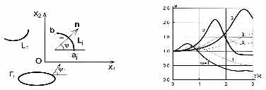
In Fig.2 there is shown the change of
quantity m = |Ts/Z| at point of the
contour of opening b = p in
the function of normalized wave number g*R = gR at J
= 0, h/R = 3, g/R = 1.5 (b is the polar angle, R is the
radius of the opening). The curve with number m is given for loading
X3 = Zsin(mb) (m = 1,2,3). The full lines
conform to variant A, the dashed ones to variant B. It is seen that by
increasing parameters in peak values g*R
dispeace to the right.
at J
= 0, h/R = 3, g/R = 1.5 (b is the polar angle, R is the
radius of the opening). The curve with number m is given for loading
X3 = Zsin(mb) (m = 1,2,3). The full lines
conform to variant A, the dashed ones to variant B. It is seen that by
increasing parameters in peak values g*R
dispeace to the right.
Concluding
remarks. The represented approach to the solution of the stationary
dynamic problem of electroelasticity permits to investigate the influence of the
inertial effect on the behaviour of the components of the electric field in a
piezoceramic space with tunnel heterogenities of a rather arbitrary
configuration. As it follow from Fig. 2 under dynamic loading quantity m may exceed its static analogue almost by 2.5 times (curve
3).
Fig.
1 Fig.
2 From the represented result of the
calculations it follows that the behaviour of the electric and mechanical
quantities considerably depend on the frequency of the harmonic loading, mutual
position and configuration of heterogenities.
The work was carried out in the framework of
an agreement on scientific cooperation between the National Technical University
of Athens and the Institute of Mechanics of the National Academy of Sciences of
Armenia.
National Technical University of
Athens, Greece
Sumy State University,
Ukraine
References
1. Nowacki W. Electromagnetic effects in solid bodies. M. Mir. 1986. 160 p. (in
Russian).
2. Maugin G.A
Continuum mechanics of electromagnetic solids. Amsterdam.
New York. North - Holland. 1988. 488 p.
3. Sih G.C. (ed.) Elastodynamic crack problems.
Leyden. Noordhoff. 1977.
4. Grinchenko V.T., Ulitko A.F., Shul'ga N.A. Electroelasticity (Mechanics of coupled fields in construction elements.
Vol.5). Kyiv. Naukova Dumka. 1989. 280 p. (in
Russian).
5. Parton V.Z.,
Kudryavtsev B.A. Electromagnetoelasticity. New York. Gordon
and Breach. 1988.
6. Bardzokas
D., Filshtinsky M.L. Electroelasticity of piecewise-uniform
bodies. Sumy (Ukraine). University Book publ. 2000. 308 p.(in
Russian).
7. Muskhelishvili N.I.
Singular Integral Equations. Groningen Wolters-Noordhoff
publishing. 1958.
8. Berlincourt
D.A., Curran D.R., Jaffe H. In: Physical acoustics. V.I.
Part A. Ed. by W.P. Mason. New-York. Academic Press.
1964.
9. Erdogan F.E., Gupta
G.D., Cook T.S. - Mechanics of Fract. Leyden. Noordhoff Int.
Pub. 1973. V.1. P. 368-425.
10. Panasyuk V.V. Savruk M.P., Nazarchuk Z.T. Method of
singular integral equations in two-dimensional diffraction problems. Kyiv.
Naukova Dumka. 1984. 344 p. (in Russian)